For my capstone project in machine learning at EPFL, I wrote a classifier capable of sorting 3D scans of archaeological objects by culture.
Digitization of museum collections is currently a major challenge faced by cultural heritage and natural history museums. Museums are expected to digitize the collections to improve not only the documentation of artifacts, but also their availability for research, reconstruction and outreach activities, and to make these digital representations available online.
Machine learning setup
While 2D-digitalization, achieved through high resolution 2D-scans and photographs, e.g. of paintings, is a well understood process, 3D-digitalization of archaeological or natural history artifacts remains costly and time-consuming: at the time of writing, digitizing an artifact can take several hours including post-processing, therefore digitization is currently reserved for the most prestigious items in the collection. Efforts towards enabling a cost-efficient and timely mass-digitization of all the artifacts in a collection are underway, e.g. at the Fraunhofer Institute for Computer Graphics Research IGD, at the Forschungs- und Kompetenzzentrum Digitalisierung Berlin and at Museum für Naturkunde Berlin.
After an artifact has been digitized, it needs to be classified in order to enable the creation of new online services for research, restoration or outreach. Classification of raw, “point cloud”, data according to a predefined typology is an open problem, and I argue that machine learning techniques offer a promising approach to solving it. When scanning a large number of artifacts (the current target at Museum für Naturkunde Berlin is several thousand each day), it becomes impractical to manually input the metadata for each 3D-model. Therefore, classification software can help to generate metadata according to a predefined typology, to enable later retrieval of the digital files.
Discussions with the digitization manager at Museum für Naturkunde Berlin (MfN) and with the contractor who provides the 3D-scanning technology at MfN show that there is a need for an automated method for extracting information from the scans. The Senate Department for Science, Research and Culture, Berlin, has setup a funding program to facilitate digitization of museum collections in Berlin, therefore the funding and employment opportunities in this sector are excellent.
Data overview
In order to train a classifier, a large data set has to be available, and it has to be labeled or described in sufficient detail. As this problem is at the cutting edge of museum technology, such datasets are scarce. Fortunately, several museums have made 3D-models of their archaeology collections available under a Creative Commons license through the Sketchfab website. These collections include many types of artifacts, but pottery (ceramics) stand out by the number of artifacts available for download.
Ceramics are an ubiquitous product of any pre-industrial culture. Ceramics have been used as containers and for transport of goods, as everyday utensils for cooking, drinking and eating, or as decorative objects, and can be found on archaeological sites in sufficient numbers to allow for statistical study.
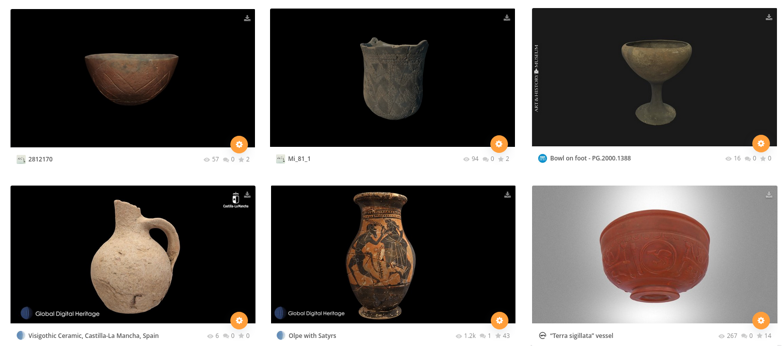
Various types of pots in the dataset: Neolithic LBK vessel, Neolithic SBK mortar, Bronze Age bowl on foot, Iron Age -Visigoth- bottle, Greek Jug, Roman cup (screenshot from the Sketchfab website).
Using the Sketchfab API, I queried the Sketchfab site and downloaded metadata describing more than thousand 3D-models, by querying Sketchfab for existing 3D-model collections and compiling new collections on my Sketchfab account. The archaeological periods and cultures present in the data set are (sorted by antiquity):
Neolithic Linear Pottery Culture (LBK), 5500–4500 BCE
A major culture widespread in Europe during the Neolithic (new stone age). LBK pottery is characteristically decorated with patterns of incised lines.
Neolithic Stroked Pottery culture (SBK), 4600-4400 BCE
The successor of the LBK. SBK pottery is characteristically decorated with patterns of punctures (dots).
Bronze Age, 3200-600 BCE (in Europe)
Characterized by standardized forms, most of which are still in use today, such as cups, pots, plates etc. Hand-made.
Iron Age, 1200-100 CE (in Europe excluding nordic countries)
Standardized forms, but made on a potters wheel.
Greek, 800 BCE- 300 BCE.
Pottery was elevated to an art form in ancient Greece. The Greek culture spans the Bronze Age (“archaic” period) and the Iron Age (“classic” period). The typology of Greek pot shapes, comprises more than a hundred standardized forms. Pottery was a medium for painting and is often decorated with sophisticated scenes.
Roman, 500 BCE-500 CE.
Technically, the Roman culture was an Iron Age culture. However, it’s common practice to classify Roman artefacts as such, due to their very recognizable forms, decorations and finishing, as well as the determining influence the Roman civilization had on other European cultures.
ML setup
The Inception v3 and MobileNet v2 are both up to the task of extracting high-level features from the data. The TF Hub implementations of MobileNet and of Inception have been trained on the ILSVRC-2012-CLS “ImageNet” data set, and have the same signature for feature vectors.
The MobileNet v2 is optimized for mobile applications. Since I’m not building a mobile application, I chose the Inception v3 model. This model expects slightly larger input images and yields 2048 features for each image.
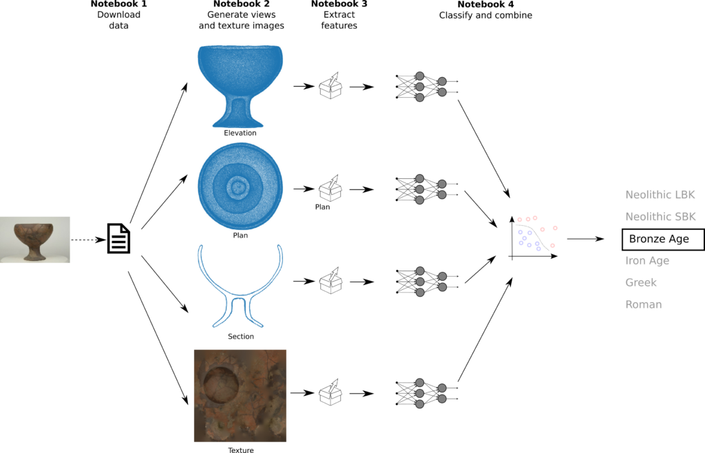
For each of the 3D-views and the texture image, I implemented a separate dense network, so there are 4 separate models to fit. Each network has 1 input and 1 output tensor, there are no branching or merging layers, so the architecture is sequential and similar for each of the 4 models:
- The input data for the network are 2048 high-level features extracted from each of the 3d-views and from the textures in the previous notebook.
- The data is not linearly separable, therefore this network needs at least one hidden layer. After some experimenting, I added two hidden layers. Choosing the number of nodes in the hidden layer is a problem for which some heuristics exist, but no definitive answer, therefore I optimize the number of nodes in the hidden layers using grid search. In this network, the second hidden layer has half the nodes of the first hidden layer.
- I added dropout layers to prevent overfitting.
- The images are in 6 classes (‘Bronze Age’, ‘Iron Age’, etc.), therefore the network requires 6 outputs.
I chose to implement the network using Keras.
The networks are trained independently from each other. There are 4 networks, one for each 3D view and one for the textures. I used grid search to optimize the accuracy of the model by tuning:
- the number of nodes in the hidden layers
- the dropout rate
- the optimizer used for compiling the model
Alternatively, I could have used cross validation for a better estimate of the parameters. However, this would be very computationally demanding, as fitting the model is itself costly, and the grid has many parameter combinations. As the data set is large enough, I did a simple grid search. Additionally, I used early stopping to reduce the computation time (this would not be compatible with cross validation).
In order to get a better estimate nonetheless,
- the train and validation data as split in notebook 1 is stratified
- the parameter class_weight is set to a dictionary of class labels per sample
- I used a batch size larger than the default
Optimizing the parameters for all 4 classifiers required about 3/4 hour on my machine, using 3 processor threads.
Conclusions
Downloading data: suitable datasets for researching this problem are rather scarce. Sketchfab proved to be a useful resource. Downloading the data set took much longer than expected, due to bandwidth limitations of the API. This particular data set has 21 GB of data.
Data processing: The data could be downloaded and processed using Python libraries, specifically the Graphics Language Transmission Format (glTF) library pygltf, the imaging library PIL and the scipy.spatial library for spatial transformations. Handling this imbalanced data set was done by stratifying the data set splits using Scikit Learn.
Extracting features: High-level features could be extracted by applying transfer learning from the Inception V2 model. This model proved capable of extracting useful features from this particular data set, although it has been trained on completely different images. As entire classes had missing texture images, I handled missing data using the imputer object provided by scikit learn.
Classification: If the F-score can be considered the most reliable metric for this particular use case, then the final scores are:
- 0.87 weighted average F-score for the k-NN classifier ensemble
- 0.84 weighted average F-score for the logistic regression classifier ensemble
The original research question was whether ML can help in the process of mass-digitization by automatically tagging scanned artifacts. This is possible, however this particular setup put 13% of the artifacts in the wrong class. Improving this score would be necessary in a production environment. Some suggestions:
- around 1000 3D-models do not seem to be enough for supervised learning
- while point clouds with tens of thousands points have enough resolution, missing textures certainly are a problem. Therefore 3D-scans should have a texture if the scanning process allows for it
- newer versions of Scikit Learn probably offer better imputer objects for missing data
- More powerful hardware (or running Keras on the GPU) would allow to run cross validation on top of grid search, which would perhaps optimize the parameters more accurately
- Changing the training strategy to training the whole setup in one go instead of each classifier in parallel could potentially improve the results, but would most certainly also require more powerful hardware
Sketchfab also has several other datasets (animal skulls, prehistoric stone tools) which could be used to deepen the understanding of this particular research question.
The Jupyter notebooks with the source code are available on GitHub.