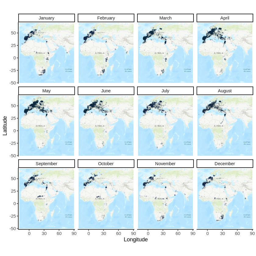
In a previous post, I discussed how to plot occurrence data from GBIF on a map. In this post, I will discuss how to plot a bird migration by producing an occurrence map for each month of the year. I will use the migration of the stork (Ciconia ciconia) as an example.

These are the libraries I will use for drawing the maps using OpenStreetMap data:

library(OpenStreetMap)
library(ggplot2)
library(sp)
library (rgdal)
library(readr)

Storks migrate from Europe where most of them breed, to southern Africa and India. The area of the map is therefore delimited by these coordinates:

LAT1 = 70 ; LAT2 = -50
LON1 = -20 ; LON2 = 90

Get the map from OpenstreetMap. A more detailed explanation of the parameters can be found here.

map <- openmap(
  c(LAT2,LON1), c(LAT1,LON2),
  zoom = 2,
  type = "esri-topo",
  mergeTiles = TRUE)
print("done loading map")

The map can now be drawn. Here, I used a longitude / latitude projection for simplicity. If you were to plot a distribution instead of occurrences, an equal area projection would be a better pick. Projection definitions can be found on the EPGS website.

# the definition of the projection
proj <- "+proj=longlat +ellps=clrk66"

# project the map
map.proj <- openproj(map, projection = proj)

# plot the map
autoplot(map.proj) +
  theme_classic() +
  labs(x="longitude", y="latitude")

Get occurrence data from GBIF, as discussed here. Save the data, without unpacking it, to file. I stored it in a file called “data/GBIF_Ciconia_ciconia.zip”. The occurrence data can now be loaded into a variable. Note that it is not necessary to unzip the file before reading it, and that the data is in tab-separated format (TSV).

The data can now be loaded and cleaned. Optionally, as the data set has 600.000 entries, I chose to sub-sample it to speed things up.

# load the file into a variable
occurrences <- read_tsv("data/GBIF_Ciconia_ciconia.zip")

# Cleanup the data
occurrences.clean <- occurrences[
  !is.na(occurrences$decimalLatitude) &
  !is.na(occurrences$decimalLongitude) &
  !is.na(occurrences$month),]

# randomly sample 25.000 entries
occurrences.sampled <-
  occurrences.clean[sample(nrow(occurrences.clean), 25000),]

Now project the data using the same projection definition as for the map

coordinates(occurrences.sampled) <- 
  c("decimalLongitude", "decimalLatitude")
proj4string(occurrences.sampled) <- CRS(proj)
occurrences.proj <- 
  spTransform(occurrences.sampled, CRS=CRS(proj))

The map and the data can now be plotted, using facets to create a map for each month of the year

# return the name of the month
month_labeller <- function(variable,value){
  return(month.name[value])
}

# plot the map and the data
autoplot(map.proj) +
  geom_count(
    data = data.frame(occurrences.proj),
    aes(x = decimalLongitude, y = decimalLatitude,
    color = ..prop..
  ), alpha=0.1, size=0.5, show.legend = FALSE
) +
scale_fill_gradient(low="red", high="yellow") +
facet_wrap(~month, labeller = month_labeller) +
theme_classic() +
labs(x="Longitude", y="Latitude")

References

GBIF.org (07 September 2020) GBIF Occurrence Download https://doi.org/10.15468/dl.vm74xx